Fine tuning Hugging Face models on Google Colab

A how-to guide for optimizing a text classification model

Aug 03, 2022

Google Colab is an interactive notebook environment for Python programming. It offers access to free or low-cost GPU computing resources for training deep learning models. Hugging Face, on the other hand, is a library of natural language models that can be fine-tuned to work on specialized NLP tasks. As I found out (in multiple ways, sadly), fine tuning these models for tasks can pose a significant set of challenges for the uninitiated.

In this post, I want to document some lessons learned from the past month or two after using Hugging Face on Google Colab for website analysis of small firm sites. I have two primary research goals: First, I want to improve the data quality of the unstructured text, such that I can, second, use it more effectively in downstream analysis. This blog focuses on the first goal of cleaning the data, but really this is just a means to an end to study small firm innovation activities.1

The website data were initially scraped and pre-processed back in 2018: You can read the details in a 2021 article published in the Journal of Official Statistics.2

Target variable

Here is an example of the data quality problem I’m trying to address in this work: If a piece of website content, e.g., a phrase or sentence, is not directly related to the study’s goals, I labeled the content with ‘0’ for discard and ‘1’ for keep. An example of garbage text is “View All”, while an example of text to retain is “We believe these parts are the wave of the future and are pleased to produce them under license from Please ask us about our PM/Series 200, 300, 400 and how they can meet your high temperature needs.” Garbage text, thus, contributes little to small firm narratives, as defined by my research objective.

Your target variable for classification could be something completely different, and you can define your label as binary or multi-class, as needed. That’s the allure of Hugging Face’s library of pre-trained models: you can download them (for free) via API and fine-tune them on a task of your choosing.

Notebook structure

Before we move on, feel free to consult the entire notebook on GitHub. It’s organized in seven sections:

Install and import libraries
EDA
Model training
Out of sample testing
Register model
Make predictions
Impute predictions into full dataset

I’m not going to document the approach and results in detail — you can contact me for a draft of the manuscript, and I’ll send it when it becomes available later this summer. Rather, I’ll focus on the non-obvious optimization steps I took, some of which are the result of using Google Colab for research purposes, others of which have to do with the computing-heavy requirements of BERT based deep learning models. These are the insights that don’t typically get published but are the most helpful to know for researchers and practitioners in their day-to-day.

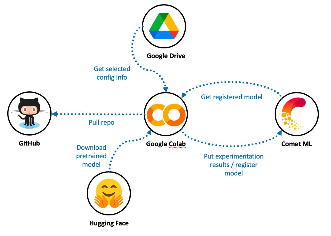
Technology architecture

In addition to using Hugging Face and Colab Pro, I rely on Comet ML as a model registry and experiment manager. Colab machines are transient, i.e., you spin them up as needed, and Google reclaims these resources after a period of inactivity. That makes tracking your experimentation progress almost impossible because the local file system goes away. We need something on the cloud that will allow us to track experimentation progress with different model specifications — and eventually, to store our champion model. Enter Comet ML.

I also use Google Drive to store some input, output, and configuration files. Colab makes it very straightforward to mount a drive upon allocating a resource, though this has to be done interactively through the notebook editor.

Note that I am using Google Colab Pro, which routinely provisions high-performance T4 and P100 GPU resources. The free version of Colab tends to offer slower machines with lower timeout thresholds.

Text classification architecture

This is a big topic and one that I can’t do justice to, given the scope of this post. But there are plenty of resources to learn about BERT-based architecture. I started with Jay Alammar’s excellent visual guide on BERT and the seminal “Attention is All You Need” paper by Vaswani et al. (2017). Then, I looked at Hugging Face’s documentation on text-classification and used O’Reilly helpful book on Scikit-Learn, Keras, and TensorFlow by Géron (2019) as a reference.

Five lessons learned

There are five main lessons I learned, and each took some time figuring out by reading the Hugging Face API and usage documentation, Stack Overflow, etc.

Setup of Comet ML
Removing duplicates from training data
Using padding and truncation in a uniform way
Avoiding overfitting
De-duplication of prediction data

1. Setup of Comet ML

Comet ML requires certain environment variables for configuration purposes. I tried multiple integration patterns, but the only one that seemed to work on Colab was to point to a .env file in my mounted Google Drive and source that using dotenv, a Python library that reads key-value pairs and sets them as environment variables. The .env file contains two variables, the Git directory for Comet’s use (COMET_GIT_DIRECTORY), as well as a pointer to the comet.config (COMET_INI) file that contains the authorization key.

This file contains bidirectional Unicode text that may be interpreted or compiled differently than what appears below. To review, open the file in an editor that reveals hidden Unicode characters. Learn more about bidirectional Unicode characters

Show hidden characters

	from comet_ml import Experiment
	from comet_ml.api import API
	from dotenv import load_dotenv

	# setup comet_ml experiment
	if IN_COLAB:
	# read env file from Google drive
	env_file = drive_path + 'MyDrive/raaste-config/.env'
	load_dotenv(env_file)

view raw comet-ml-setup.py hosted with ❤ by GitHub

2. Removing duplicates from training data

I hand-labeled 5,624 observations using the target variable criteria above (i.e., keep or discard). Surprisingly, I didn’t realize until later that there were hundreds of duplicates. A duplicate might consist of commonly used website text, such as “View All” or “Click to learn more”. During model training, retaining duplicate training and validation observations felt like cheating because BERT models have many weights, some of which could become overly sensitive to repeat observations. Indeed, removing duplicates initially led to lower model performance on the validation data.

3. Using padding and truncation in a uniform way

From what I can tell, there are separate ways to create datasets for training and validation vs. inference. Inference here means predicting outcomes on your out-of-sample dataset for final model evaluation, plus the other non-labeled data, which as you’ll read more below, totaled over 2 million observations.

Padding and truncation are needed after tokenizing the raw text and transforming the tokens to their embedding representations. This is because BERT-based models, and in general sequential models running on GPUs, expect fixed sentence lengths. In my case, I set the truncation and padding lengths to 100 tokens. This means that sentences longer than 100 tokens get truncated and sentences with fewer than 100 tokens get padded. I won’t get into the details here, but here are the different ways prep the data for training and validation vs. the inference pipeline.

3.1. Creating batched tf datasets for training and validation

Notice how tokenization and padding happens with different function references when creating the tf datasets.

Show hidden characters

	# set batch size
	bs = 64

	# base bert checkpoint -- load tokenizer
	checkpoint = "bert-base-uncased"
	tokenizer = AutoTokenizer.from_pretrained(checkpoint)

	# non_null_df is a pandas dataframe
	dataset = Dataset.from_pandas(non_null_df, split='train')
	dataset.cast_column(target, datasets.Value('int8'))

	# 85% train, 15% test + validation
	train_test_dataset = dataset.train_test_split(test_size=0.15)
	# Split the 20% test + valid in half test, half valid
	test_valid_dataset = train_test_dataset['test'].train_test_split(test_size=0.3)
	# gather everyone if you want to have a single DatasetDict
	train_test_valid_dataset = datasets.DatasetDict({
	'train': train_test_dataset['train'],
	'test': test_valid_dataset['test'],
	'valid': test_valid_dataset['train']})

	# tokenize with truncation
	def tokenize_function(x):
	return tokenizer(x["sample_text"], truncation=True, max_length=100)

	tokenized_dataset = train_test_valid_dataset.map(tokenize_function, batched=True, batch_size=None)

	# add padding
	data_collator = DataCollatorWithPadding(tokenizer=tokenizer, padding="max_length", max_length=100, return_tensors="tf")

	tf_train_dataset = tokenized_dataset["train"].to_tf_dataset(
	columns=["attention_mask", "input_ids", "token_type_ids"],
	label_cols=target,
	shuffle=True,
	collate_fn=data_collator,
	batch_size=bs,
	)

	tf_validation_dataset = tokenized_dataset["valid"].to_tf_dataset(
	columns=["attention_mask", "input_ids", "token_type_ids"],
	label_cols=target,
	shuffle=False,
	collate_fn=data_collator,
	batch_size=bs,
	)

view raw tokenize-padding.py hosted with ❤ by GitHub

3.2. Performing inference with padding and tokenization

I tried to get inference working with the test dataset above, but all the examples I found used string lists fed into inference pipelines. In this type of usage, you have to set the padding and tokenization specifications as configuration inputs.

Show hidden characters

	# get list of strings and list of labels
	eval_text = train_test_valid_dataset['test']['sample_text']
	eval_labels = train_test_valid_dataset['test'][target]

	# define inference pipeline
	pipe = pipeline ("text-classification", model=model, tokenizer=tokenizer, device=0, batch_size = 8,function_to_apply='sigmoid' )
	tokenizer_kwargs = {'padding':'max_length','truncation':True,'max_length':100}

	# run pipeline
	out = pipe (eval_text, **tokenizer_kwargs)

view raw inference-pipeline.py hosted with ❤ by GitHub

4. Avoiding overfitting

Overfitting may be addressed by reducing model size and implementing dropout and label smoothing. There are other techniques, as well, such as changing your optimizer, but the steps below were fairly effective for me.

The baseline configuration for a Hugging Face model consists of twelve attention heads, twelve hidden layers, an input vector size of 768 going into each hidden layer, and an intermediate hidden layer size of 3,072. This is a very large model spec given the number of training and validation observations available. Initial model training and validation showed significant overfitting, in that taining loss would decline after each epoch while validation loss would increase. In contrast, with a pared-down model architecture, the model showed a reduced tendency to overfit. The winning architecture was smaller in size:

config.hidden_size = 32 config.intermediate_size = 128 config.num_hidden_layers = 4 config.num_attention_heads = 4

Additional configuration changes were made by increasing the default dropout rates of 0.1 for hidden and attention layers to 0.2:

config.hidden_dropout_prob = 0.2 config.attention_probs_dropout_prob = 0.2

Finally, label smoothing was applied as a regularization technique to avoid overfitting on the binary 0 or 1 classification labels. Keras makes label smoothing particularly easy to implement in the loss function, which here is Binary Focal Cross-entropy.

loss = BinaryFocalCrossentropy(from_logits=True, label_smoothing=0.2)

5. De-duplication of prediction data

There were over two million text snippets for which I needed classification predictions. I would keep those with a predicted label of 1, i.e., those exceeding a sigmoid value of 0.5, and discard the rest. It turns out that millions of predictions, even when batched in the pipeline, easily overwhelm Colab Pro resources. Rather than divide up the prediction workload into multiple itereations, I turned to de-duplicating the input text, running predictions on just about 200+ thousand unique text phrases, and storing the results in a hash map. Running inference using a GPU for the 200+ thousand predictions took over 5 hours. I stored the results to file on my Google Drive so that I could access them later in another Colab session.

Finally, I iterated on the initial dataset of 2 million observations and looked up the predicted value in the hash map, after which I retained or discarded the text based on the predicted class. This step only took a few seconds.

Conclusion

The out of sample evaluation results produced an accuracy score of 0.939 — not bad for a binary classification problem for two relatively well-balanced classes. Upon closer inspection of the results, ‘misclassified’ observations in the test set could have been coded as worthy or garbage (i.e., there was some ambiguity in the real label type) or were in fact initially improperly coded.

There’s a lot more going on here than what I cover in this post, but most of that falls into the bucket of relatively straightforward machine learning best practices and architectural patterns. The above discussion, while not comprehensive, contains tricks that would have saved me a ton of time in training and selecting a high performing model. I hope this guide will help you out with the same aim in mind. Good luck!

And, of course, feel free to post any insights that will clarify or correct the content.

A Reasonable Mind

Discussion about this post

Ready for more?